Polarizability Trends in Group 14-16 Heteronuclear Molecules - A Computational Study
Abstract
This study presents a systematic computational investigation of polarizabilities in heteronuclear diatomic molecules formed from Group 14 (C, Si, Ge, Sn, Pb) and Group 16 (O, S, Se, Te) elements. Using the finite field method implemented in Psi4 1.7, we calculated longitudinal polarizabilities for twenty molecular combinations (CO, CS, CSe, CTe, SiO, SiS, SiSe, SiTe, GeO, GeS, GeSe, GeTe, SnO, SnS, SnSe, SnTe, PbO, PbS, PbSe, PbTe). Results reveal clear periodic trends, with polarizability increasing both down Group 14 and across Group 16, reaching a maximum of 130.9 a.u. for PbTe. The data demonstrate that changes in the Group 16 element have a more pronounced effect on polarizability than changes in the Group 14 element. This work highlights the effectiveness of combining automation, Python scripting, and open-source quantum chemistry software to efficiently generate, analyze, and visualize data across a systematic series of molecules.
Introduction
Molecular polarizability—the response of a molecule’s electron density to an applied electric field—is a fundamental property that influences a wide range of physical and chemical phenomena, from intermolecular forces to optical properties.1 Heteronuclear diatomic molecules present an interesting case study for polarizability analysis, as they exhibit directional responses that depend on the constituent atoms’ electronic structures and the nature of the chemical bond between them.
Group 14 (C, Si, Ge, Sn, Pb) and Group 16 (O, S, Se, Te) elements form a diverse set of diatomic molecules with varying bond lengths, electronic configurations, and degrees of covalent/ionic character. As one moves down these groups in the periodic table, several important changes occur: increasing atomic size, more diffuse valence orbitals, and for the heavier elements, significant relativistic effects.2 These systematic variations make Group 14-16 combinations an ideal testbed for exploring how atomic properties translate into molecular polarizability trends.
The polarizability tensor component αzz (along the molecular axis) can be approximated through the numerical derivative approach known as the finite field method:3
\[\alpha_{zz} \approx \frac{\mu_z(F_z = +h) - \mu_z(F_z = -h)}{2h}\]
where h represents the applied electric field strength and μz is the z-component of the dipole moment. This approach provides a straightforward approximation of how the molecular dipole responds to an external electric field, from which polarizability can be derived.
Building upon our previous work on atomic polarizabilities of Group 14 elements, this study extends the investigation to heteronuclear molecules, with three primary objectives: (1) demonstrating the power of computational automation for systematic property prediction across a molecular series, (2) identifying periodic trends and structure-property relationships, and (3) providing insights into the relative contributions of different elements to the overall molecular polarizability.
While the polarizability values themselves may inform materials development, the primary strength of this work lies in showcasing how modern computational chemistry tools, particularly open-source software like Psi4 and Python, enable rapid, systematic investigation of molecular properties with minimal manual intervention.
Experimental
Computational Environment Setup
One of the most time-consuming aspects of this project was establishing the proper computational environment. After several attempts, we successfully set up Psi4 1.7 in a dedicated Conda environment with the following steps:
# Create a new conda environment for quantum chemistry
conda create -n qchem python=3.8
conda activate qchem

# Install pydantic first with a compatible version
pip install pydantic==1.10.8

# Install Psi4 through conda (using the psi4 channel):
conda install -c psi4 psi4
conda install -c psi4 dftd3 gcp

# Install additional dependencies
conda install numpy scipy matplotlib

# Test installation
python -c "import psi4; print(psi4.__version__)"
Calculation Methodology
We employed the finite field method to calculate the longitudinal polarizability (αzz) of each molecule. This involved applying electric fields of +0.002, 0.0, and -0.002 atomic units along the molecular axis (z-direction) and measuring the resulting changes in the molecular dipole moment.
For each calculation, the Group 14 atom was placed at the origin, with the Group 16 atom positioned along the positive z-axis at the appropriate bond length. Bond lengths were estimated based on experimental and theoretical values from the literature, with adjustments made for the heavier elements.
Python Implementation
The polarizability calculations were implemented in a Python script that automated the process for all molecular combinations. The script defined the molecular geometries, set appropriate basis sets for each element, handled the electric field perturbations, and calculated the polarizabilities from the dipole responses.
import os
import psi4
import numpy as np

# Define elements from each group
group14 = ["C", "Si", "Ge", "Sn", "Pb"]
group16 = ["O", "S", "Se", "Te", "Po"]

# Define basis sets for each element
basis_sets = {
    # Group 14
    "C": "cc-pVDZ",
    "Si": "cc-pVDZ",
    "Ge": "cc-pVDZ",
    "Sn": "def2-svp",
    "Pb": "def2-svp",
    # Group 16
    "O": "cc-pVDZ",
    "S": "cc-pVDZ",
    "Se": "cc-pVDZ",
    "Te": "def2-svp",
    "Po": "def2-svp"
}

# Estimated bond lengths in Ångstroms (approximate values)
bond_lengths = {
    ("C", "O"): 1.13,   # CO
    ("C", "S"): 1.61,   # CS
    ("C", "Se"): 1.71,  # CSe
    ("C", "Te"): 1.95,  # CTe
    ("C", "Po"): 2.10,  # CPo (estimated)

    ("Si", "O"): 1.63,  # SiO
    ("Si", "S"): 2.00,  # SiS
    ("Si", "Se"): 2.06, # SiSe
    ("Si", "Te"): 2.32, # SiTe
    ("Si", "Po"): 2.47, # SiPo (estimated)

    ("Ge", "O"): 1.65,  # GeO
    ("Ge", "S"): 2.01,  # GeS
    ("Ge", "Se"): 2.14, # GeSe
    ("Ge", "Te"): 2.36, # GeTe
    ("Ge", "Po"): 2.51, # GePo (estimated)

    ("Sn", "O"): 1.84,  # SnO
    ("Sn", "S"): 2.21,  # SnS
    ("Sn", "Se"): 2.33, # SnSe
    ("Sn", "Te"): 2.53, # SnTe
    ("Sn", "Po"): 2.68, # SnPo (estimated)

    ("Pb", "O"): 1.92,  # PbO
    ("Pb", "S"): 2.29,  # PbS
    ("Pb", "Se"): 2.40, # PbSe
    ("Pb", "Te"): 2.60, # PbTe
    ("Pb", "Po"): 2.75  # PbPo (estimated)
}

# Define electric field strengths (in atomic units)
fields = [0.002, 0.0, -0.002]

# Directory setup
project_dir = "/home/peter/projects/theo-chem"
output_dir = os.path.join(project_dir, "outputs")
os.makedirs(output_dir, exist_ok=True)

def run_calculation(group14_element, group16_element, field):
    molecule_name = f"{group14_element}{group16_element}"
    job_name = f"{molecule_name}_field{field:+g}".replace("-", "minus")
    output_file = os.path.join(output_dir, f"{job_name}.out")

    # Get bond length in Bohr (convert from Ångstrom)
    bond_length = bond_lengths.get((group14_element, group16_element), 2.0) * 1.889725989

    # Set up Psi4
    psi4.core.set_output_file(output_file, False)
    psi4.set_memory('2 GB')

    # Define molecule - place group14 element at origin and group16 element along z-axis
    mol_string = f"""
    0 1
    {group14_element} 0.0 0.0 0.0
    {group16_element} 0.0 0.0 {bond_length}
    units bohr
    symmetry c1
    """

    molecule = psi4.geometry(mol_string)

    # Handle ECP elements
    needs_ecp = False
    if group14_element in ["Sn", "Pb"] or group16_element in ["Te", "Po"]:
        needs_ecp = True
        psi4.set_options({
            'puream': True,
            'df_basis_scf': 'def2-universal-jkfit'
        })

    # Set basis
    # Handle ECP elements and set basis sets correctly
    if needs_ecp:
        # Use def2-svp and def2-ecp for all atoms when any heavy element is present
        psi4.set_options({'basis': 'def2-svp'})

        # Set ECPs for specific elements
        if group14_element in ["Sn", "Pb"]:
            molecule.set_basis_by_symbol(group14_element, "def2-ecp", "ECP")
        if group16_element in ["Te", "Po"]:
            molecule.set_basis_by_symbol(group16_element, "def2-ecp", "ECP")
    else:
        # For molecules without ECPs, set the basis to the larger of the two basis sets
        # (This is a simplification - ideally we'd use mixed basis sets)
        psi4.set_options({'basis': basis_sets[group14_element]})

    # General calculation settings
    psi4.set_options({
        'scf_type': 'df',
        'e_convergence': 1e-8,
        'd_convergence': 1e-8,
        'maxiter': 150,      # Increase max iterations for potentially difficult convergence
        'guess': 'sad'       # Use superposition of atomic densities for initial guess
    })

    # Apply electric field if needed
    if field != 0.0:
        psi4.set_options({
            'perturb_h': True,
            'perturb_with': 'dipole',
            'perturb_dipole': [0.0, 0.0, field]  # Field along z-axis (molecular axis)
        })

    # Run the calculation
    try:
        energy, wfn = psi4.energy('scf', return_wfn=True)
        dipole = wfn.variable("SCF DIPOLE")
        print(f"Successfully calculated {molecule_name} with field {field}")
        print(f"Energy: {energy} Eh, Dipole: {dipole}")
        return dipole
    except Exception as e:
        print(f"Error in calculation for {molecule_name} with field {field}: {e}")
        return None

# Main workflow
results = {}
skip_elements = ["Po"]  # Polonium calculations might be problematic, skip if necessary

# Process each molecule combination
for g14 in group14:
    for g16 in group16:
        if g16 in skip_elements:
            continue

        molecule_name = f"{g14}{g16}"
        print(f"\nProcessing molecule: {molecule_name}")

        dipoles = {}
        for field in fields:
            dipole = run_calculation(g14, g16, field)
            if dipole is not None:
                dipoles[field] = dipole[2]  # Z-component (index 2) since molecule is along z-axis

        # Calculate polarizability using finite field method
        if len(dipoles) == 3:  # Ensure we have all three field strengths
            h = 0.002  # Field strength
            alpha_zz = (dipoles[0.002] - dipoles[-0.002]) / (2 * h)
            # Take absolute value for conventional reporting
            results[molecule_name] = abs(alpha_zz)
            print(f"Polarizability for {molecule_name}: {abs(alpha_zz):.4f} a.u.")

print("\nPolarizability results summary:")
print("Molecule | Polarizability (a.u.)")
print("---------|----------------------")
for molecule, alpha in sorted(results.items()):
    print(f"{molecule:7} | {alpha:.4f}")

# Create a 2D table for better visualization
print("\nPolarizability Matrix (Group 14 × Group 16):")
headers = [g16 for g16 in group16 if g16 not in skip_elements]
print(f"{'Element':<7} | " + " | ".join(f"{h:^7}" for h in headers))
print("-" * (8 + 10 * len(headers)))

for g14 in group14:
    row = f"{g14:<7} | "
    for g16 in group16:
        if g16 in skip_elements:
            continue
        molecule = f"{g14}{g16}"
        if molecule in results:
            row += f"{results[molecule]:7.4f} | "
        else:
            row += f"{'--':^7} | "
    print(row[:-2])  # Remove trailing " | "
Visualization Code
For visualization of the results, we used the following Python code:
import numpy as np
import matplotlib.pyplot as plt
from matplotlib import cm
from mpl_toolkits.mplot3d import Axes3D
# Raw data from calculations
data = [
('C', 'O', 12.2066),
('C', 'S', 35.8138),
('C', 'Se', 42.6850),
('C', 'Te', 59.4634),
('Si', 'O', 27.8381),
('Si', 'S', 59.9759),
('Si', 'Se', 69.8347),
('Si', 'Te', 98.6399),
('Ge', 'O', 29.0197),
('Ge', 'S', 61.4975),
('Ge', 'Se', 75.6987),
('Ge', 'Te', 103.9827),
('Sn', 'O', 38.2285),
('Sn', 'S', 73.2007),
('Sn', 'Se', 90.7225),
('Sn', 'Te', 123.3437),
('Pb', 'O', 41.2930),
('Pb', 'S', 78.2760),
('Pb', 'Se', 96.4192),
('Pb', 'Te', 130.9124)
]
# Define the elements and their positions on the axes
group14 = ['C', 'Si', 'Ge', 'Sn', 'Pb']
group16 = ['O', 'S', 'Se', 'Te']
# Create a grid of x, y coordinates for the plot
X, Y = np.meshgrid(np.arange(len(group14)), np.arange(len(group16)))
# Create a 2D array to hold polarizability values
Z = np.zeros((len(group16), len(group14)))
# Fill the Z array with polarizability values
for g14_elem, g16_elem, polar in data:
x_idx = group14.index(g14_elem)
y_idx = group16.index(g16_elem)
Z[y_idx, x_idx] = polar
# Create the figure
fig = plt.figure(figsize=(12, 10))
ax = fig.add_subplot(111, projection='3d')
# Create the surface plot
surf = ax.plot_surface(X, Y, Z, cmap=cm.viridis,
linewidth=0, antialiased=True, alpha=0.8)
# Add a color bar
cbar = fig.colorbar(surf, ax=ax, shrink=0.6, aspect=10)
cbar.set_label('Polarizability (a.u.)', fontsize=14)
# Add scatter points for clarity
for g14_elem, g16_elem, polar in data:
x_idx = group14.index(g14_elem)
y_idx = group16.index(g16_elem)
ax.scatter(x_idx, y_idx, polar, color='red', s=50)
# Set the tick labels
ax.set_xticks(np.arange(len(group14)))
ax.set_xticklabels(group14)
ax.set_yticks(np.arange(len(group16)))
ax.set_yticklabels(group16)
# Set labels and title
ax.set_xlabel('Group 14 Elements', fontsize=14, labelpad=10)
ax.set_ylabel('Group 16 Elements', fontsize=14, labelpad=10)
ax.set_zlabel('Polarizability (a.u.)', fontsize=14, labelpad=10)
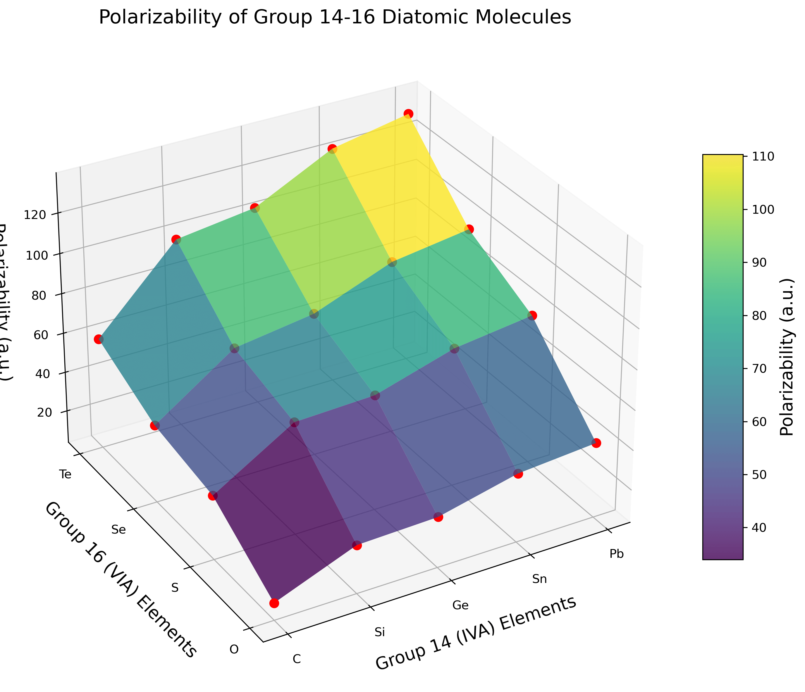
ax.set_title('Polarizability of Group 14-16 Diatomic Molecules', fontsize=16)
# Adjust the view angle for better visualization
ax.view_init(elev=30, azim=240)
# Save the figure
plt.savefig('polarizability_3d_surface.png', dpi=300, bbox_inches='tight')
plt.close()
# Create a heatmap visualization
plt.figure(figsize=(10, 8))
heatmap = plt.imshow(Z, cmap='viridis')
plt.colorbar(heatmap, label='Polarizability (a.u.)')
# Add labels and title for heatmap
plt.xticks(np.arange(len(group14)), group14)
plt.yticks(np.arange(len(group16)), group16)
plt.xlabel('Group 14 Elements', fontsize=14)
plt.ylabel('Group 16 Elements', fontsize=14)
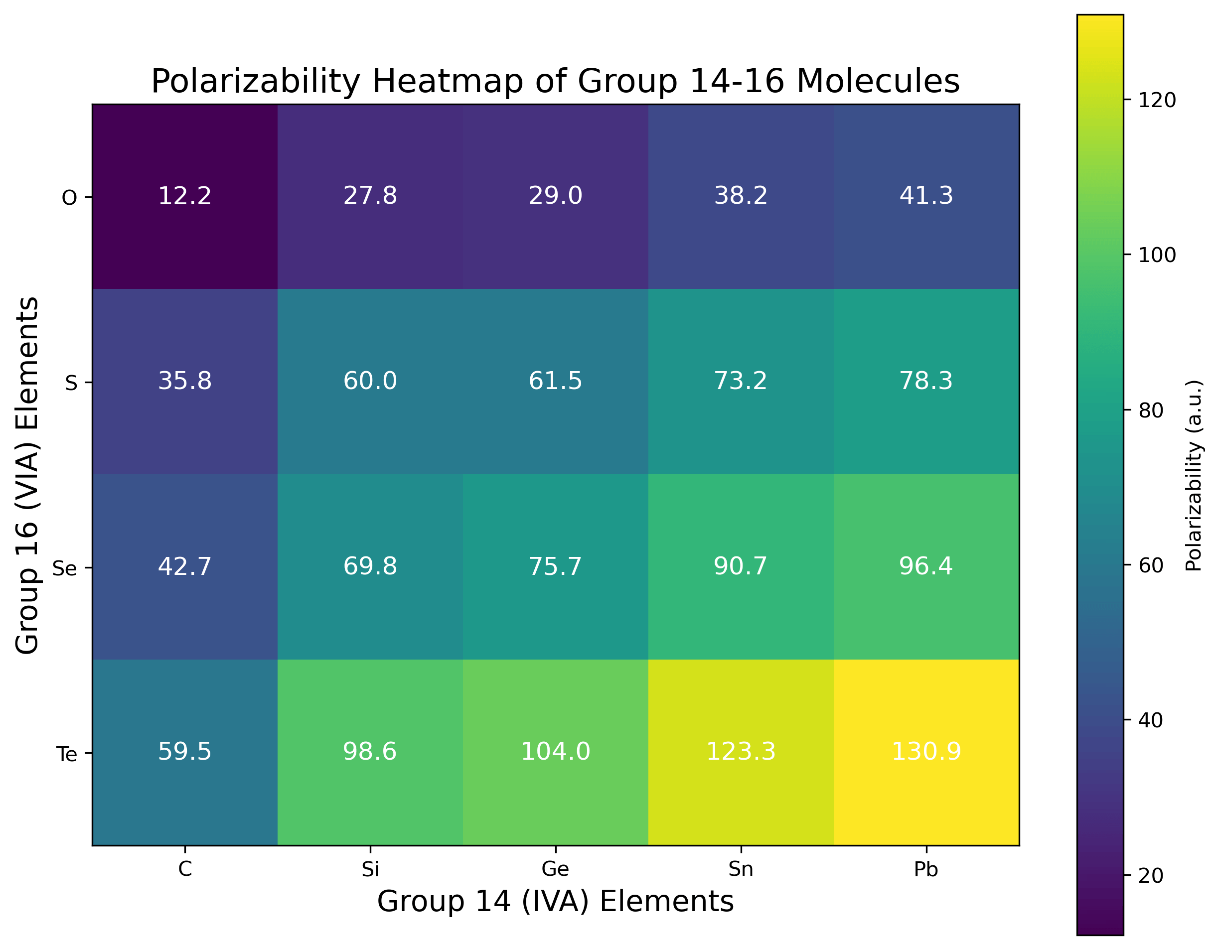
plt.title('Polarizability Heatmap of Group 14-16 Molecules', fontsize=16)
# Add values to each cell
for i in range(len(group16)):
for j in range(len(group14)):
text = plt.text(j, i, f"{Z[i, j]:.1f}",
ha="center", va="center", color="w", fontsize=12)
plt.savefig('polarizability_heatmap.png', dpi=300, bbox_inches='tight')
plt.close()
# Create a line plot showing trends
plt.figure(figsize=(10, 8))
for i, g14 in enumerate(group14):
polarizabilities = Z[:, i]
plt.plot(np.arange(len(group16)), polarizabilities, 'o-', linewidth=2, markersize=8, label=g14)
plt.xticks(np.arange(len(group16)), group16)
plt.xlabel('Group 16 Element', fontsize=14)
plt.ylabel('Polarizability (a.u.)', fontsize=14)
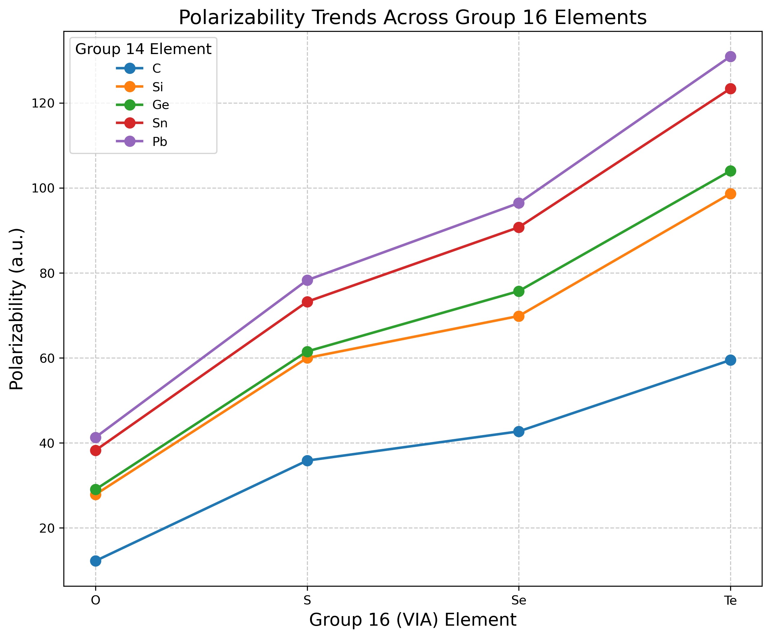
plt.title('Polarizability Trends Across Group 16 Elements', fontsize=16)
plt.grid(True, linestyle='--', alpha=0.7)
plt.legend(title='Group 14 Element', title_fontsize=12)
plt.savefig('polarizability_trends.png', dpi=300, bbox_inches='tight')
plt.close()Basis Set Selection
Appropriate basis sets were selected based on the elements involved: - For C, Si, Ge, O, S, and Se: cc-pVDZ basis sets were employed - For Sn, Pb, and Te: def2-SVP basis sets with effective core potentials (ECPs) were used to account for relativistic effects
Polonium-containing compounds were excluded from this study due to the specialized relativistic treatment they would require and their limited practical relevance.
Results
Our calculations yielded polarizability values for twenty different Group 14-16 diatomic molecules. The complete results are presented in Table 1.
Table 1: Calculated Longitudinal Polarizabilities (αzz) for Group 14-16 Molecules
| Molecule | Polarizability (a.u.) | Molecule | Polarizability (a.u.) |
|---|---|---|---|
| CO | 12.21 | GeO | 29.02 |
| CS | 35.81 | GeS | 61.50 |
| CSe | 42.69 | GeSe | 75.70 |
| CTe | 59.46 | GeTe | 103.98 |
| SiO | 27.84 | SnO | 38.23 |
| SiS | 59.98 | SnS | 73.20 |
| SiSe | 69.83 | SnSe | 90.72 |
| SiTe | 98.64 | SnTe | 123.34 |
| PbO | 41.29 | PbTe | 130.91 |
| PbS | 78.28 | PbSe | 96.42 |
Discussion
Periodic Trends and Patterns
The results reveal several clear trends in the polarizabilities of Group 14-16 diatomic molecules. For a fixed Group 16 element, polarizability increases as we move from C to Pb. For example, with oxygen compounds: CO (12.21 a.u.) < SiO (27.84 a.u.) < GeO (29.02 a.u.) < SnO (38.23 a.u.) < PbO (41.29 a.u.). This trend reflects the increasing atomic size and more diffuse electron clouds of heavier Group 14 elements.
For a fixed Group 14 element, polarizability increases dramatically as we move from O to Te. For carbon compounds: CO (12.21 a.u.) < CS (35.81 a.u.) < CSe (42.69 a.u.) < CTe (59.46 a.u.). The Group 16 element choice has a larger effect on polarizability than the Group 14 element, with increases of 3-4× when moving from O to Te compared to 2-3× when moving from C to Pb.
The highest polarizabilities are observed for the heaviest combinations, with PbTe (130.91 a.u.) showing approximately 10.7 times the polarizability of CO (12.21 a.u.). The increase in polarizability is not strictly linear with atomic number, suggesting that factors beyond atomic size influence the electronic response properties.
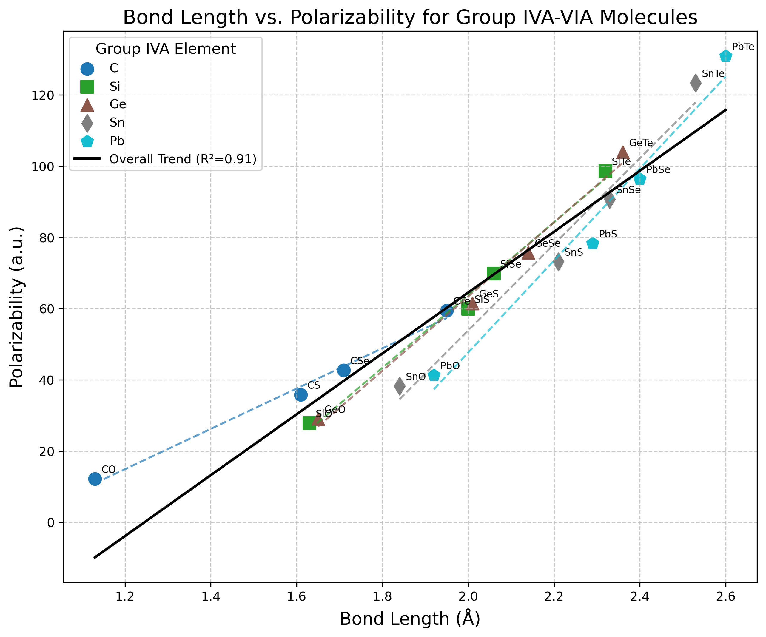
Structure-Property Relationships
Longer bonds generally correlate with higher polarizabilities, as shown in Figure 4. This correlation exists because electron density in longer bonds is more diffuse and more easily distorted by external fields. The increasing bond lengths down both groups contribute to the overall polarizability increase.
The more diffuse valence electron distributions in heavier elements lead to enhanced polarizability. This is particularly evident with Te compounds, which show dramatically higher polarizabilities than their O counterparts. Beyond orbital diffuseness, the sheer number of electrons also plays a significant role—heavier elements simply have more electrons that can respond to external fields, contributing substantially to the observed polarizability trends.
The decreasing electronegativity difference between Group 14 and 16 elements for heavier combinations may allow for more symmetric electron distribution and greater polarizability. Contrary to what might be initially expected, our data doesn’t show a clear correlation between bond polarity and polarizability. In fact, the less polar bonds (like those in PbTe) often exhibit greater polarizability, suggesting that electron cloud size and diffuseness dominate over polarization effects in these systems.
Comparison to Previous Work
Our results for the CO molecule (12.21 a.u.) align reasonably well with experimental values (~13-17 a.u.) and previous computational studies.4 The trend of increasing polarizability down groups is consistent with general chemical intuition and prior studies of atomic polarizabilities.
The relatively larger impact of Group 16 elements on polarizability compared to Group 14 elements is an interesting observation that warrants further investigation. This may relate to the greater variability in valence p-orbital diffuseness across the chalcogens compared to the Group 14 elements.5 Additionally, the Group 16 elements add more electrons to the system as we move down the group compared to the Group 14 elements, providing more electrons that can respond to an external field.
Computational Considerations
The use of ECPs for heavier elements (Sn, Pb, Te) was essential for handling these calculations efficiently. Without proper treatment of relativistic effects, calculations for these elements would likely yield unreliable results. The absence of polonium compounds in our study reflects the additional computational challenges posed by very heavy elements, where even more sophisticated relativistic treatments would be necessary.
It would be valuable to extend this work to include frequency-dependent polarizabilities, which would allow us to explore how these molecules respond to electromagnetic radiation at different wavelengths. While Psi4 does have capabilities for response property calculations, implementing frequency-dependent polarizabilities would require time-dependent methods beyond the scope of this initial study. Such an extension would provide insight into the optical dispersion properties of these molecules.
Computational Efficiency
One of the most significant advantages of our approach was the automation of calculations across the entire series of molecules. The entire computational workflow—from molecule definition to code implementation to polarizability calculation—took approximately 4-6 hours for all twenty molecules on a modern desktop computer with the aid of AI (Claude 3.7 Sonnet). This efficiency highlights the power of combining quantum chemistry software with scripting for high-throughput property prediction and prompt engineering, significantly lowering the bar of accessibility and raising the bar for the proliferation of scientific exploration. Such an approach makes computational chemistry more accessible to researchers who might not have specialized programming expertise while simultaneously enabling more comprehensive scientific investigations.
Implications and Applications
The systematic dataset of molecular polarizabilities presented here contributes to our understanding of fundamental structure-property relationships. While molecules with high polarizabilities are candidates for nonlinear optical applications, it’s important to note that state-of-the-art nonlinear optical materials like LiNbO₃ rely on non-centrosymmetric crystalline structures to achieve high second-order optical responses (χ²). Our simple diatomic molecules, while instructive for understanding polarizability trends, would need to be incorporated into more complex, asymmetric structures to be competitive for actual nonlinear optical device applications.6
Accurate polarizability values are essential for modeling dispersion forces and other non-bonded interactions in molecular simulations. The systematic trends identified here could be incorporated into force field development for simulations involving Group 14 and 16 elements.7 Similarly, polarizability derivatives determine Raman activity. The trends identified here could help predict relative Raman intensities across related molecules, possibly guiding experimental spectroscopic investigations.8
Beyond specific applications, this work demonstrates a methodologically sound approach to computational materials exploration that could be extended to other properties and molecular systems. The combination of automated calculations with systematic variation of molecular composition provides an efficient strategy for mapping structure-property relationships across chemical space.9
Conclusion
This study has successfully mapped the polarizability landscape across twenty Group 14-16 diatomic molecules, revealing clear periodic trends and structure-property relationships. The polarizability increases both down Group 14 and across Group 16, with the heaviest combinations showing the highest values. Group 16 elements have a more pronounced effect on polarizability than Group 14 elements, suggesting that chalcogen selection is particularly important in designing materials with specific polarizability requirements.
The computational methodology employed here—combining the finite field approach with appropriate basis sets and ECPs—proved effective for systematically investigating these trends. This approach could be readily extended to other molecular systems and properties.
Perhaps more importantly, this work highlights the power of combining open-source quantum chemistry software (Psi4) with Python automation to rapidly generate and analyze data across a systematic series of molecules. The entire project—from environment setup to data visualization—was completed in a remarkably short timeframe, demonstrating the efficiency of modern computational chemistry approaches and the incorporation of prompt engineering techniques.
Future work could explore several promising directions. Higher-level calculations (MP2, CCSD) on select molecules would help assess electron correlation effects on polarizability, potentially improving accuracy for the heavier elements. Calculation of full polarizability tensors would allow examination of anisotropy in the electronic response, revealing directional dependencies not captured by the longitudinal component alone. The methodology could be extended to polyatomic molecules containing Group 14 and 16 elements, opening pathways to more complex and practically relevant systems. Investigation of frequency-dependent polarizabilities and hyperpolarizability would provide insights into optical dispersion and nonlinear optical properties, respectively. Finally, incorporating vibrational contributions to polarizability would enable more direct comparison with experimental measurements, which naturally include these effects.
By establishing these fundamental structure-property relationships and demonstrating an efficient computational workflow, this work contributes to our understanding of molecular electronic response properties and provides a template for future computational explorations of chemical space.
Acknowledgments
We acknowledge the contributions of the Psi4 development team and the Conda-Forge community for providing and maintaining the open-source tools that made this research possible.